SimCLR-S2 Stage 1: Pretraining
Contents

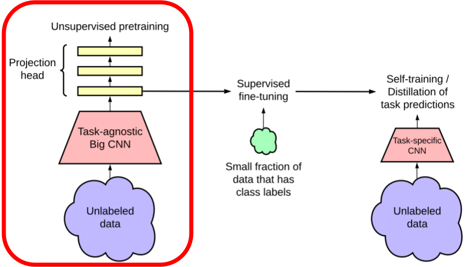
In this post, we will explore the first phase of the SimCLR methodology, pretraining. As stated previously, pretraining leverages unlabeled data by performing a pair of augmentations on a batch of raw images. With the augmented batch, we train a model on a large task agnostic convolutional neural network to maximize the agreement between the images. The image pairs derived from the same base are said to attract each another while repel all other images in the batch.
Augmentation Techniques
Before any training can commence, we needed to determine how and which augmentations to apply to our satellite images. To identify which augmentations were the most effective, we performed a series of training runs with different combinations of augmentations and ran fine-tuning on the resulting models. Exhaustive training runs were completed with random couplets of the augmentations described in Table 1.
| Pixel Augmentations | Geometric Augmentations |
|---|---|
| blur | flip |
| brightness | rotation |
| contrast | shift |
| gain | zoom |
| speckle |
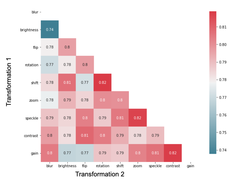
Figure 1 shows the various augmentations used and the corresponding F1 score of the resulting fine-tuned model. Training was performed on 3% of the data to improve iteration time in running experiments. Based on the results, it was inconclusive which augmentations produced the most effective pre-trained model so we decided to remove the bottom 25% of the augmentations from the average score to be used for the full training runs.

Figure 1: F1 scores of fine-tuned models based on applied pretraining augmentations. The figure represents the average score between the regular and extended labels.
Training
California and Big Earth Net data were both used for pretraining. Due to the California dataset’s smaller size, all hyperparameter tuning for pretraining leveraged that data set. Resource constraints limited the ability to perform robust experimentation of hyperparameters, so experiments were limited to learning rate and optimizer.
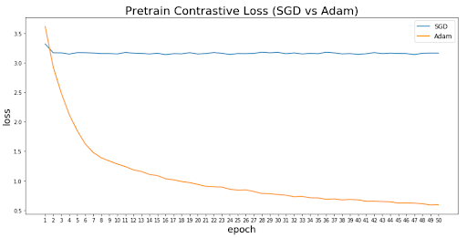
Figure 2 shows the result of using an adam optimizer versus stochastic gradient descent (SGD). When using the adam optimizer, the loss seems to decrease even toward the end for the training epochs continually. SGD, conversely, seems to flatten after only three epochs.

Figure 2: Pretraining loss curves compairing SGD versus adam optimizers.
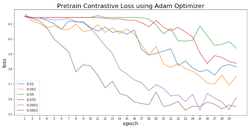
Since the adam optimizer seemed to be a clear winner due to the loss curve, we chose it for learning rate experiments. The learning rate experiments used varying values between 0.0001 and 0.05. Figure 3 summarizes the learning rate results and shows that the ideal rate among the samples is 0.0005.

Figure 3: Loss curves for various learning rates using the adam optimizer on the Californina data set.
After all hyperparamter tuning experiments were completed, full training was conducted with parameters summarized in Table 2.
| Parameter | Value |
|---|---|
| Architecture | ResNet152 |
| Batch Size | 32 |
| Epochs | 50 |
| Temperature | 0.1 |
| Optimizer | adam |
| Learning Rate | 0.0005 |