Exploratory Analysis
Contents
We perform an exploratory analysis on our data to get better insights into understanding the distributions for irrigated land in our labeled data set and identifying potential features that might enhance our ability to distinguish between permanently irrigated land from those that are not. We also explore pre-processing techniques that will help our models learn better from the data and analyze image augmentations that are more suited to satellite images in the context of irrigation detection
The BigEarthNet-S2 data set covers images from ten European countries: Austria, Belgium, Finland, Ireland, Kosovo, Lithuania, Luxembourg, Portugal, Serbia, Switzerland. These images are annotated with multiple labels. Cultivated land under agricultural use that are either permanently or periodically irrigated, using a permanent infrastructure like irrigation channels, drainage network, spray sprinkler line, rotary sprinkler and additional irrigation facilities are labeled with Permanently irrigated land. Most of these crops cannot be cultivated without artificial water supply. And these labels do not include sporadically irrigated land. This label is our target label. Only 2.3% of the images in our data are labeled as Permanently irrigated land.
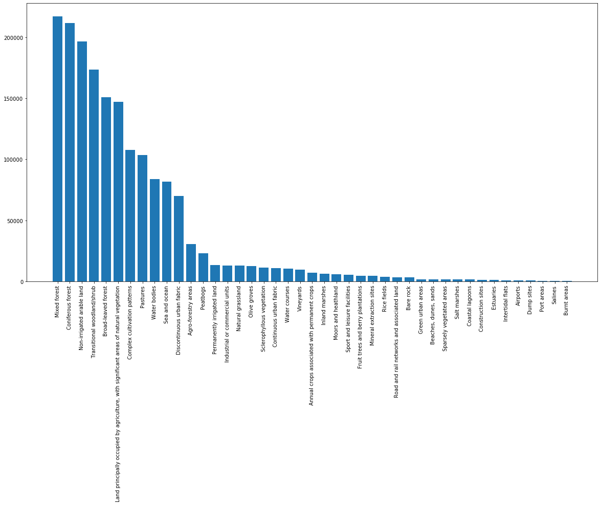
Figure 1: Distribution of labels in BigEarthNet-S2
Further reading on the Corine land cover nomenclature showed that there were permanent crops which also potentially included permanently irrigated land and hop plantations but were covered under a different class label. These include Vineyards, Fruit trees and berry plantations, Olive groves and Rice fields
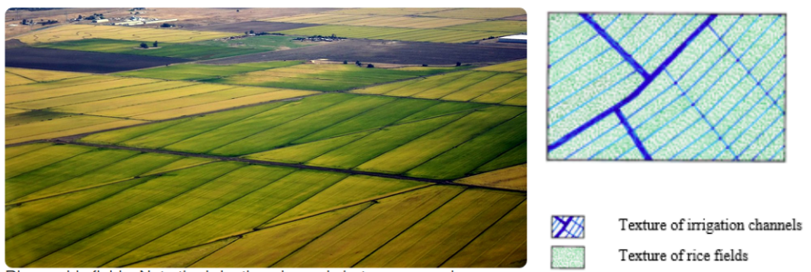
Figure 2: Rice fields with the irrigation channels between parcels
Clubbing these above land classes with permanently irrigated land puts the percentage of potentially irrigated land at 6.2%. In our experiments, we compare and contrast our learnings from the pure target labels with those from the extended target labels to see if the latter helps generalize our models better.

Figure 3: Statistics of irrigated land with additional labels
Vegetation and Water Canopy Indices
Remote sensors aboard satellites measure wavelengths of light absorbed and reflected by land surfaces. Pigments like chlorophyll, found in plant leaves, strongly absorb wavelengths of visible red light and strongly reflect wavelengths of near-infrared light. As plant canopy changes with seasons, these reflectance properties also change. Vegetation index is a transformation of two or more spectral bands designed to serve as an indication of health of vegetation for each pixel in a satellite image. There are several vegetation indices, of which, we studied a handful during our EDA.
Enhanced vegetation Index (EVI)
EVI is an optimized vegetation index designed to enhance the vegetation signal with improved sensitivity in high biomass regions. A de-coupling of the canopy background signal and a reduction in atmosphere influences gives an improved vegetation monitoring. Typically EVI uses three bands: the red, blue and near infra-red. However, the blue band has often found to be problematic, with a poor signal to noise ratio. This is mainly due to the nature of the reflected energy in this part of the spectrum over land, which is extremely low. EVI is therefore computed using two bands following this equation:
$$ EVI= \frac{2.5 \times (NIR−Red)}{NIR+ (2.4 \times Red) +1} $$
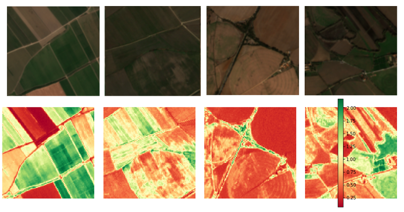
Figure 4: Visual bands (top) and EVI (bottom) for irrigated samples from BigEarthNet data
Soil Adjusted Vegetation Index (SAVI)
Normalized Differential Vegetative Index (NDVI) is sensitive to the effects of soil and atmosphere. SAVI is an adjusted form of widely used NDVI, developed to minimize the influence of soil brightness on spectral vegetation indices, particularly in areas of high soil composition. A soil adjustment factor L is added to the equation of NDVI to correct for soil noise effect like soil color, soil moisture etc.
$$ SAVI = \frac{(NIR – Red)}{(NIR + Red + L)} \cdot (1 + L) $$
L is a variable in $(-1, 1)$ and its value depends on the amount of green vegetation present in the area.

Figure 5: SAVI for irrigated samples from BigEarthNet data
Moisture Stress Index (MSI)
The Mositure Stress Index (MSI) is a reflectance measurement that is sensitive to the increasing leaf water content. As the water content of leaves in vegetation canopies increases, the strength of the absorption around 1600 nm (SWIR or band 11) increases. Absorption at 819 nm (NIR or band 8) is nearly unaffected by changing water content, so it is used as the reference. The MSI is inverted relative to the other water vegetative indices; higher values indicate greater water stress and less water content.
$$ MSI = \frac{MIR}{NIR} $$
Normalized Difference Infrared Index (NDII)
NDII is a reflectance measurement that is sensitive to changes in water content of plant canopies. The NDII uses a normalized difference formulation instead of a simple ratio as used in MSI. The index values increase with increasing water content. Applications include crop agricultural management, forest canopy monitoring, and vegetation stress detection. The formula for computing thsi index is shown below:
$$ NDII=\frac{(NIR−MIR)}{(NIR+MIR)} $$

Figure 6: NDII for irrigated samples from BigEarthNet data
Normalized Multi-band Drought Index (NMDI)
This index, also sometime referred to as Normalized Difference Water Index or NDWI, takes into account a soil moisture background to monitor potential drought conditions. Three specific bands were chosen because of their unique response to variations in soil and vegetation moisture. The index uses the difference between two liquid-water absorption bands in the shortwave-infrared region (1640 and 2130 nm) as a measure of water sensitivity in vegetation and soil. As soil moisture increases, the index values decrease. Index values range from 0.7 to 1 for dry soil, 0.6 to 0.7 for soil with intermediate moisture, and less than 0.6 for wet soil.
$$ NMDI=\frac{(NIR−(SWIR1−SWIR2))}{(NIR+(SWIR1−SWIR2))} $$

Figure 7: NMDI for irrigated samples from BigEarthNet data
These vegetation and water canopy indices are often highly correlated with one another, as evidenced in many of our image samples, a couple of which are shown below.

Figure 8: Correlation matrix of vegetation and water canopy indices
Image Pre-processing
We observe that standardizing images increases the ability to distinguish features that are typically closer together. The below images and histograms are an attempt to visualize what this process does to image readability by adjusting the levels of the image pixels. In this example, we have standardized the pixels by computing the mean and standard deviation of a specific band 8 image from BigEarthNet-S2 dataset: S2A_MSIL2A_20170613T101031_29_89_B08.tif. The pre-processing improves the readability, as evidenced by the image and its histogram, on the right.
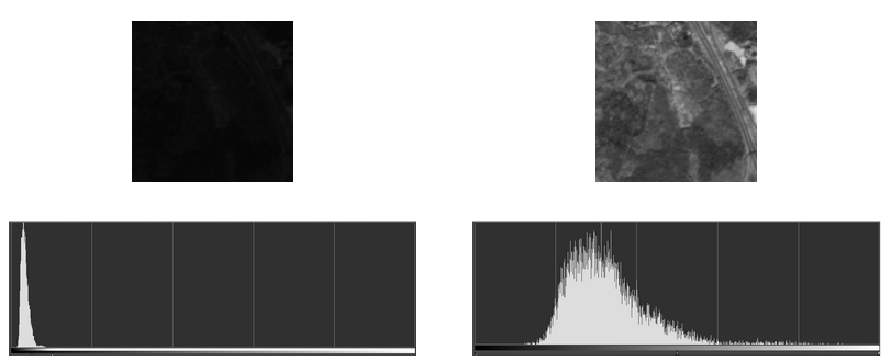
Figure 9: Effect of standardizing images on a band 8 image. Original image (left), Standardized Image (right)
For our experiments, however, we used the mean and the standard deviation computed for each band, by dataset, to scale down the scores to a common range. While we calculated the mean and the standard deviations for images that formed our California dataset, we used the provided statistics for BigEarthNet-S2.
Image Augmentation
Image augmentation is a salient feature of the SimCLR pretrain step, where every raw image in a batch is subject to two transformations before we compute the similarity between these transformed images in the batch. During the exploratory analysis, we experimented with 9 different augmentation techniques to determine which ones would be most effective on Sentinel-2 images, given that we have 10 channels per image. We studied the following augmentations: rotate, flip, zoom, shift, blur, brightness, gain, contrast and speckle. The effect of some of these per pixel transformations are discussed below.
Brightness
The brightness of an image can be augmented either darkening or brightening the images, or both. This type of transformation allows a model to generalize across images trained on different lighting levels. Brightness is an additive operation and shifts the image pixel values to the left or right.
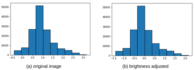
Figure 10: Histogram showing effects of brightness adjustment causing the scale to shift to the right in this example
Contrast
Contrast is adjusted independently for each channel of the image. For a contrast factor $cf$, this operation computes the mean of the image pixels in the channel and then adjusts each component x of each pixel to $(x - mean) * cf + mean$. Contrast adjustment analyzes the distribution of pixel densities in an image and then rescales the image to include all intensities that fall within a given range of intensities. For e.g. the 5th and 95th percentiles, as evidenced in image below.
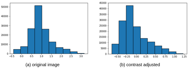
Figure 11: Histogram showing effects of contrast adjustment, with factor 0.5, causing the counts to move closer to the mean.
Gamma or Gain
Every pixel in an image has a brightness level called luminance. This value ranges between 0 and 1 where 0 indicates complete darkness and 1 indicates fully bright. Different sensors and video devices capture luminance differently and therefore a correction is applied using the formula $Out = gain * In**gamma$ where $In$ is the original pixel value, $Out$ is the output pixel value and $gamma$ is correction factor and $gain$ is a scalar multiplier. Gamma operation is not symmetric about the mean as evidenced in the figure 12 below

Figure 12: Effects of gamma adjustment causing the mean to shift to the left in this example
Gamma factor less than 1 causes an image to be darker while a value greater than 1 causes an image to be brighter, as demonstrated by the images below.
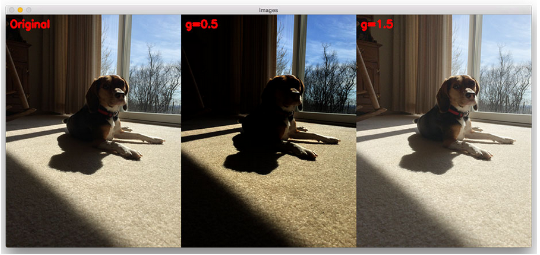
Figure 13: Effects of gamma factor on brightness of an image